Duplication in your data can lead to errors in calculations, statistics, or data visualization. Removing duplication is the first step in ensuring the integrity of your data.
Excel is one of the most popular and versatile spreadsheet applications in the world. Excel can be used for a variety of purposes, from data analysis and report generation to information management. However, one problem often faced by Excel users is duplicates in their data.
A duplicate is the same or similar data that appears more than once in one or more columns or rows. Duplicates can cause calculation errors, data inconsistencies, or decreased Excel performance.
To avoid those problems, you need to know how to remove duplicates in Excel easily and quickly. There are several ways you can use to remove duplicates in Excel, depending on your needs and preferences. In this article, we will discuss three main ways to remove duplicates in Excel, namely:
- Use the “Remove Duplicates” features available in Excel
- Use “COUNTIF” or “COUNTIFS” formulas to mark duplicates
- Use “Pivot Table” to filter out duplicates
Let’s look at each of them in more detail.
Using the Remove Duplicates Feature
The easiest and fastest way to remove duplicates in Excel is to use the “Remove Duplicates” feature available in Excel. This feature allows you to select the columns or rows that you want to remove duplicates, and then delete all the same or similar data in those columns or rows. The following are the steps to use the “Remove Duplicates” feature:
- Select all the data you want to deduplicate. You can use the shortcut “Ctrl + A” to select all data in a worksheet, or click and drag the mouse to select a specific range of data.
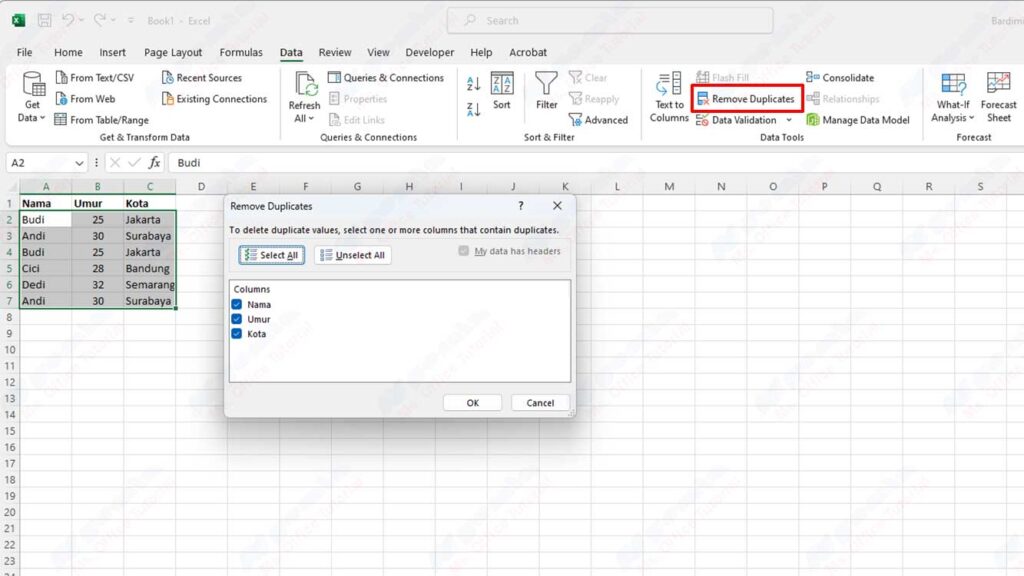
- Click the “Data” tab on the ribbon, then click the “Remove Duplicates” button in the “Data Tools” group.
- In the “Remove Duplicates” dialog box, select the column or row that you want to remove duplicates. You can select more than one column or row by pressing the “Ctrl” key when clicking the column or row name. If you want to remove duplicates based on all columns or rows, check the “Select All” box.
- Click the “OK” button to remove duplicates. Excel will display a message telling you how many duplicates have been removed and how much unique data is left.
- Click the “OK” button again to close the dialog box.
For example, suppose you have the following data:
| Name | Age | City |
| Budi | 25 | Jakarta |
| Andi | 30 | Surabaya |
| Budi | 25 | Jakarta |
| Cici | 28 | Bandung |
| Dedi | 32 | Semarang |
| Andi | 30 | Surabaya |
If you want to remove duplicates based on the Name column, then you can do as following steps:
- Select all the data, and then click the “Remove Duplicates” button on the “Data” tab.
- In the “Remove Duplicates” dialog box, check the Name column, then click the “OK” button.
- Excel will display a message dialog box that there are 2 duplicates removed and 4 unique data remaining.
- Click the “OK” button to close the dialog box.
Note that Excel only deletes rows that have the same value in the Name column, regardless of the value in the other columns. If you want to remove duplicates based on more than one column, for example, the Name and Age columns, then you can check both columns in the “Remove Duplicates” dialog box.
This feature “Remove Duplicates” is very useful if you want to permanently remove duplicates from your data. However, there are a few things you need to pay attention to when using this feature, namely:
- This feature will remove duplicates directly from your original data, without making copies or backups first. Therefore, we recommend that you make a copy of your data before using this feature, or use the “Undo (Ctrl + Z)” feature if you want to undelete duplicates.
- This feature can only remove duplicates that are the same, excluding duplicates that have differences in upper or lower case letters, spaces, or punctuation. For example, “Budi” and “budi” won’t be considered duplicates by this feature. If you want to remove duplicates that have these differences, you’ll need to take a few extra steps, such as using “UPPER”, “LOWER”, or “TRIM” formulas to equalize the format of your data before using “Remove Duplicates” feature.
- This feature can only remove duplicates in one worksheet, excluding duplicates existing in other worksheets in the same or different workbooks. If you want to remove duplicates existing in other worksheets, you need to copy or move those data to the same worksheet first or use other ways we will discuss below.
Using the COUNTIF or COUNTIFS Formula
The second way to remove duplicates in Excel is to use the formula “COUNTIF” or “COUNTIFS”. This formula can be used to count the number of times a value appears in one or more columns or rows. Using this formula, you can mark duplicates by providing specific values, such as 1 for unique data and 0 for duplicate data. Then, you can filter or remove the data marked as duplicate according to your need. The following are the steps to use the “COUNTIF” or “COUNTIFS” formula:
- Select all the data you want to deduplicate. You can use the shortcut “Ctrl + A” to select all data in a worksheet, or click and drag the mouse to select a specific range of data.
- Select an empty cell to the right or bottom of your data, depending on whether you want to mark duplicates based on columns or rows.
- Type the formula “COUNTIF” or “COUNTIFS” according to the criteria you want. “COUNTIF” formulas are used to mark duplicates based on a single column or row only, while “COUNTIFS” formulas are used to mark duplicates based on more than one column or row. The general format of this formula is as follows:
=COUNTIF(range,criteria)
=COUNTIFS(criteria_range1,criteria1,criteria_range2,criteria2,...)
Where:
- range is the range of cells that you want to count the number of times a value appears in it.
- criteria is the value you want to find in that range of cells. You can use direct values, cell references, or logical expressions to define criteria. For example, “Budi”, A2, or “>25”.
- criteria_range1, criteria_range2,… is the range of cells that you want to use as criteria to mark duplicates. You can use more than one range of cells by separating them with commas.
- criteria1, criteria2,… is the value you want to search in that range of criteria cells. You can use direct values, cell references, or logical expressions to define criteria.
- Press the “Enter” button to display the formula result. If the result is more than 1, there are duplicates in your data. If the result is 1, the record is unique. If the result is 0, the data doesn’t exist in the range of cells you specified.
- Repeat steps 3 and 4 for all records that you want to mark duplicates. You can use the “Fill (Ctrl + R)” or “(Ctrl + D” ) feature to fill formulas to other cells automatically.
- After all data is marked with formulas, you can filter or delete the data that has a value of 0 or more than 1 according to your need. You can use the “Filter” feature on the “Data” tab to filter data by a specific value or use the “Sort” feature on the “Home” tab to sort data by a specific value. Then, you can delete the unwanted data by pressing the “Delete” button.
For example, suppose you have data as in the previous table.
If you want to mark duplicates based on the Name column, then you can do as following steps:
- Select the entire data, and then select the blank cell to the right of your data.
- Type the formula =COUNTIF($A$2:$A$7,A2) in the blank cell. This formula counts the number of times the value in cell A2 appears in the range A2:A7. If the value appears more than once, then it is a duplicate. If the value appears only once, then it is unique data.
- Press the “Enter” button to display the formula result. Here, the result is 2, because there are two “Budi” in the Name column.
- Repeat steps 2 and 3 for all records that you want to mark duplicates. You can use the “Fill” feature to fill formulas to other cells automatically.
- After all, data is marked with formulas, you can filter or delete the data that has values over 1 according to your needs. For example, if you want to filter unique data, then you can use the “Filter” feature to select only 1 value in the formula field.
As a result, your data will look like this:
| Name | Age | City | Formula |
| Budi | 25 | Jakarta | 2 |
| Andi | 30 | Surabaya | 2 |
| Budi | 25 | Jakarta | 2 |
| Cici | 28 | Bandung | 1 |
| Dedi | 32 | Semarang | 1 |
| Andi | 30 | Surabaya | 2 |
Use Pivot Tables
The third way to remove duplicates in Excel is to use “Pivot Table”. Pivot Table is a feature that can be used to summarize, analyze, and present data as dynamic tables. By using Pivot Tables, you can easily filter data based on specific criteria, including removing duplicates. The following are the steps to use a Pivot Table:
- Select all the data you want to deduplicate. You can use the shortcut “Ctrl + A” to select all data in a worksheet, or click and drag the mouse to select a specific range of data.
- Click the “Insert” tab on the ribbon, then click the “PivotTable” button in the “Tables” group.
- In the “Create PivotTable” dialog box, select the location where you want to place the Pivot Table. You can select a location within the same worksheet, a new worksheet, or a new workbook.
- Click the “OK” button to create a Pivot Table.
- On the “PivotTable Fields” pane, select the column or row that you want to use as criteria for removing duplicates. You can select more than one column or row by pressing the “Ctrl” key when clicking the column or row name. Then, drag the column or row name to the “Rows” or “Columns” area of the “PivotTable Fields” pane.
- On the “PivotTable Fields” pane, select the column or other row you want to display in the Pivot Table. Then, drag the column or row name to the “Values” area of the “PivotTable Fields” pane.
- On the “PivotTable Fields” pane, select the other columns or rows that you want to filter to filter data based on specific values. Then, drag the column or row name to the “Filters” area of the “PivotTable Fields” pane.
- In the created Pivot Table table, you can view the filtered data based on the criteria you selected. Data that has the same or similar values in a criteria column or row is merged into a single row or column only, so there are no duplicates in the data.
- If you want to change the criteria or filters used to filter data, you can click the small arrow button next to the column or row name in the Pivot Table table, and then choose the option you want from the menu that appears.
- If you want to delete the Pivot Table and return to your original data, you can click the “Analyze” tab on the ribbon, then click the “Clear” button on the “Actions” group, and choose the “Clear All” option.
For example, suppose you have data as in the previous table:
If you want to remove duplicates based on Name and Age columns, then you can do as following steps:
- Select all the data, and then click the “PivotTable” button on the “Insert” tab.
- In the “Create PivotTable” dialog box, select the location where you want to place the Pivot Table. For example, select a new worksheet.
- Click the “OK” button to create a Pivot Table.
- In the “PivotTable Fields” pane, select the Name and Age columns, and then drag the column names to the “Rows” area of the “PivotTable Fields” pane.
- In the “PivotTable Fields” pane, select the City column, and then drag the column name to the “Values” area of the “PivotTable Fields” pane.
- In the created Pivot Table table, you can see the filtered data by Name and Age columns. Data that has the same or similar values in that column is combined into a single row, so there are no duplicates in the data.
Other Ways to Remove Duplicates in Excel
In addition to the three ways we have discussed above, there are several other ways you can use to remove duplicates in Excel, namely:
- Use “Conditional Formatting” to highlight duplicates of a specific color, and then filter or delete the highlighted data.
- Use “Advanced Filter” to filter unique data, and then copy or move that data to another location.
- Use “VBA” (Visual Basic for Applications) to create a macro that can remove duplicates automatically by using specific code.
These methods may require some additional steps or special knowledge to do so but can provide results that are more flexible or fit your needs. You can find more information about these ways on the internet or in Excel guidebooks.
Thus the article we made about how to remove duplicates in Excel. We hope this article has helped you manage your data better and more efficiently. Thank you for reading this article.