How to Create a Chart with Hidden Data in Excel

Hiding chart data in Excel is beneficial for securing the data and adding to a better view.

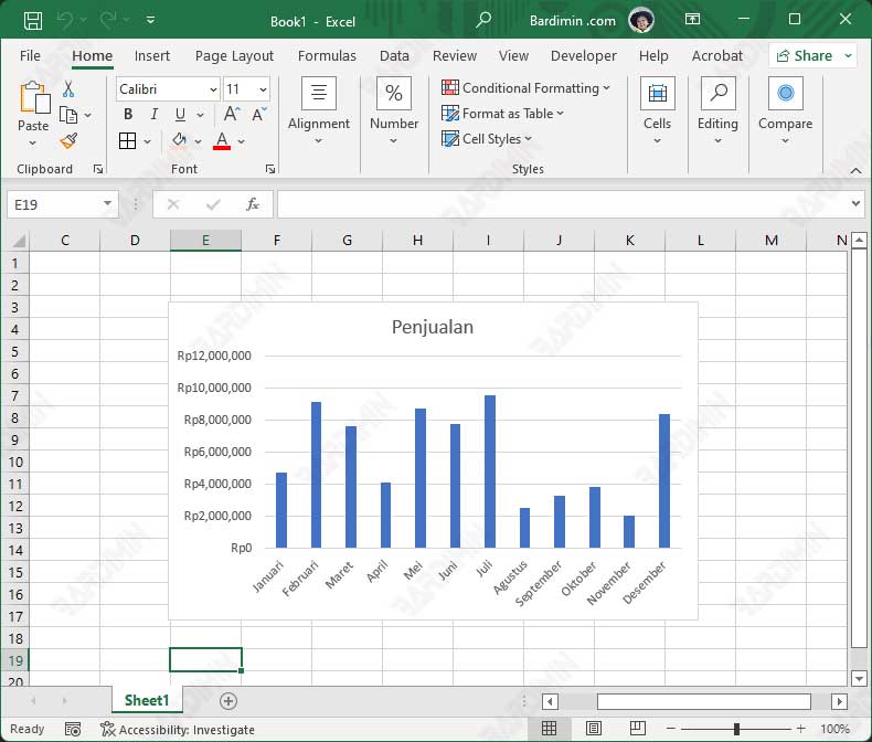
A chart is a graphical representation of data in columns and rows. Using Charts will help you visualize your data in a way that is easily understood by your audience. Typically, charts are used to analyze trends and patterns in data sets.

For example, let’s say you have data on sales figures in Excel for several years. Using the Chart, you can easily determine which year has the highest and lowest sales. You can also create charts to compare specific goals with actual results.

Microsoft Excel is very effective for analyzing trends and patterns in large amounts of data because it is easy to layout, reformat, and rearrange data, process data, and examine charts and graphs.

Excel can allow users to display information graphically so that the audience can easily understand it. You can even personalize the Chart in Excel by changing the color or rearranging the position of the data in the Chart.

Sometimes you may need to secure data or display less information on the Chart. Hiding chart data will also help you show the Chart more simply and look nicer. If you hide chart data, you will see only charts.

How to Show Chart with Hidden Data in Excel

When you hide rows or columns of data, the Chart will no longer show that data by default, and Excel will not show it on the Chart.

To display a chart with hidden data in Excel, follow the instructions below.

A. Create the Dataset

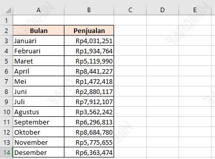
To show how we’ll be using the sales dataset for a few months.

B. Create a Chart in Excel

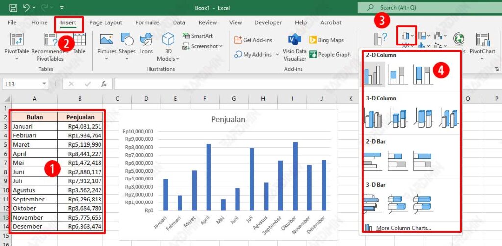
1. Dataset Selection in the previous step.
2. Then select the “Insert” tab on the Ribbon.
3. Click the “Insert Column or Bar Chart” icon button.
4. Select the chart view you want.

C. Hiding Chart Data in Excel

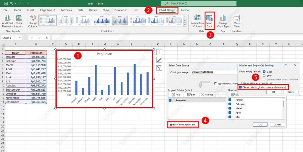
1. Click the Chart you created earlier.
2. Then select the “Chart Design” tab on the Ribbon.
3. Click the “Select Data” icon button.
4. In the dialog box, click “Hidden and Empty Cells”.
5. Then in the next dialog box, check the checkbox “Show data in hidden rows and columns”.
6. Click the OK button on all dialog boxes.

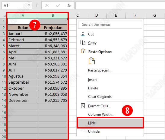
Next is the step to hide the dataset.

7. Dataset column selection (in the figure, selection of columns A and B).
8. Right-click and select the “Hide” option.

Next, you will see a view of the Chart with hidden data as shown below.

If you hide chart data without using steps like the example, the chart will not show any chart or be blank.