PivotTables are a feature in Microsoft Excel that can organize and study data. This tool can help you find patterns, trends, and comparisons in your data.
If you have a lot of data in Excel, Pivot Table helps you create a summary quickly and easily. It can organize, calculate, and analyze data in many different ways. Pivot tables can help you organize and understand large amounts of data. However, many people find it difficult to understand.
Pivot Tables make it easy to create and modify summary tables. You can do this by moving the columns from the original table. It’s this turnaround or moves that make this feature gets its name.
Pivot tables can be changed or rotated to view data in a new way. When you use pivots, you don’t do anything to your data such as add or remove. Instead, all you’re doing is organizing the information in a way that can display useful details.
Simply put, a Pivot Table understands a set of numbers on your computer. This tool helps you organize your information in different ways to make it easier to understand.
Create a Pivot Table
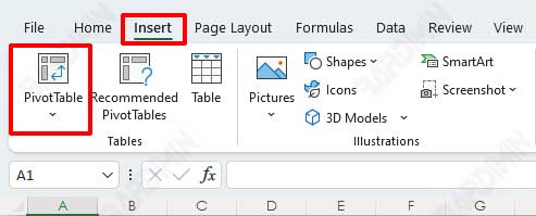
To create a Pivot Table, follow the steps presented in the PivotTable Wizard. You can access this wizard on the “Insert” tab and then click the “PivotTable” button as shown below.
1] Specify the location of Pivot Table data
After you open the PivotTable Wizard under “Insert > PivotTable”, you will see a wizard dialog box like the following.
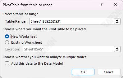
In this step, you determine the source of the data that you will analyze. Excel can work with different types of data for Pivot Tables.
When you use the wizard, you will find various pop-up windows based on the data source located. These sections show the boxes that the wizard uses to gather information from an Excel list or database.
You can use a variety of sources to get information on a Pivot Table, such as Excel databases, outside data sources, various tables, and other Pivot Tables.
Data sources in a Microsoft Excel worksheet
The data source that you will analyze is usually an Excel worksheet. The database stored in a worksheet has a limit of 1,048,576 rows and 16,384 columns. Working with a database of this size is inefficient and there may be insufficient RAM. The first row in the database must contain the field names. There are no other rules. Data can consist of values, text, or formulas.
External data sources
If you want to create a Pivot Table with data from another database, use a tool called Query to get that data. You can use different types of data on your computer such as dBASE files, SQL Server data, or any other type set up for use by your computer. You can also create a Pivot Table from an OLAP database.
Specify the location of a Pivot Table
In this step, you also specify the location of the Pivot Table you created, see the bottom of the dialog box. You can create a Pivot Table on a new worksheet or current worksheet. If you select the current worksheet, you can specify the start cell of the Pivot Table.
2] Setting the Pivot Table Layout
After you specify the data location and click the OK button, you will get a dialog box as the below screenshot shown in your specified worksheet (PivotTable location).
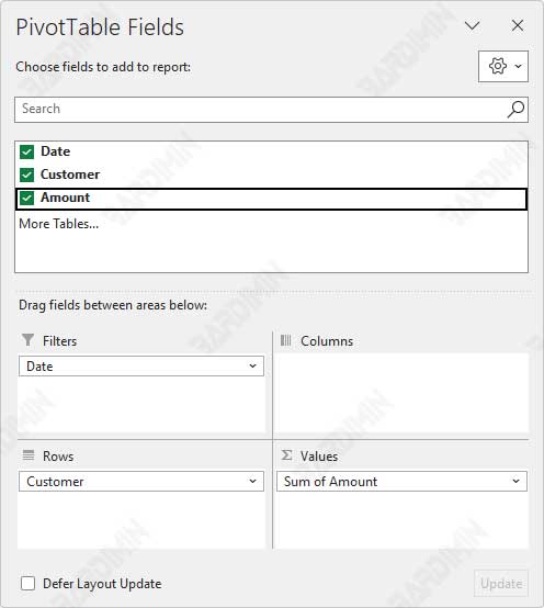
Column headings in the database appear as buttons at the top of the dialog box. Drag the buttons to the appropriate area of the Pivot Table dialog box.
The Pivot Table dialog box has four areas:
“Filters”: The buttons in this area appear as displayed data filter items.
“Rows”: Buttons in this area appear as row items in the Pivot Table.
“Columns”: The buttons in this area appear as column items in the Pivot Table
“Values”: The buttons in this area indicate the data summarized in the Pivot Table.
You can move multiple buttons where you want and you don’t have to put them all. If you don’t use some data, it won’t appear in the Pivot Table.
If you move the button to the “Values” area, the PivotTable sums the values if they are numbers, or counts the numbers if they are not numbers.
When you create a Pivot Table, you can double-click on the button to change it as you want. You can choose how to calculate or summarize specific fields. You can choose the things you want to hide in a category. If you move a button to the wrong place, you can remove it from the table by dragging it. You can change the fields in the Pivot Table whenever you want.
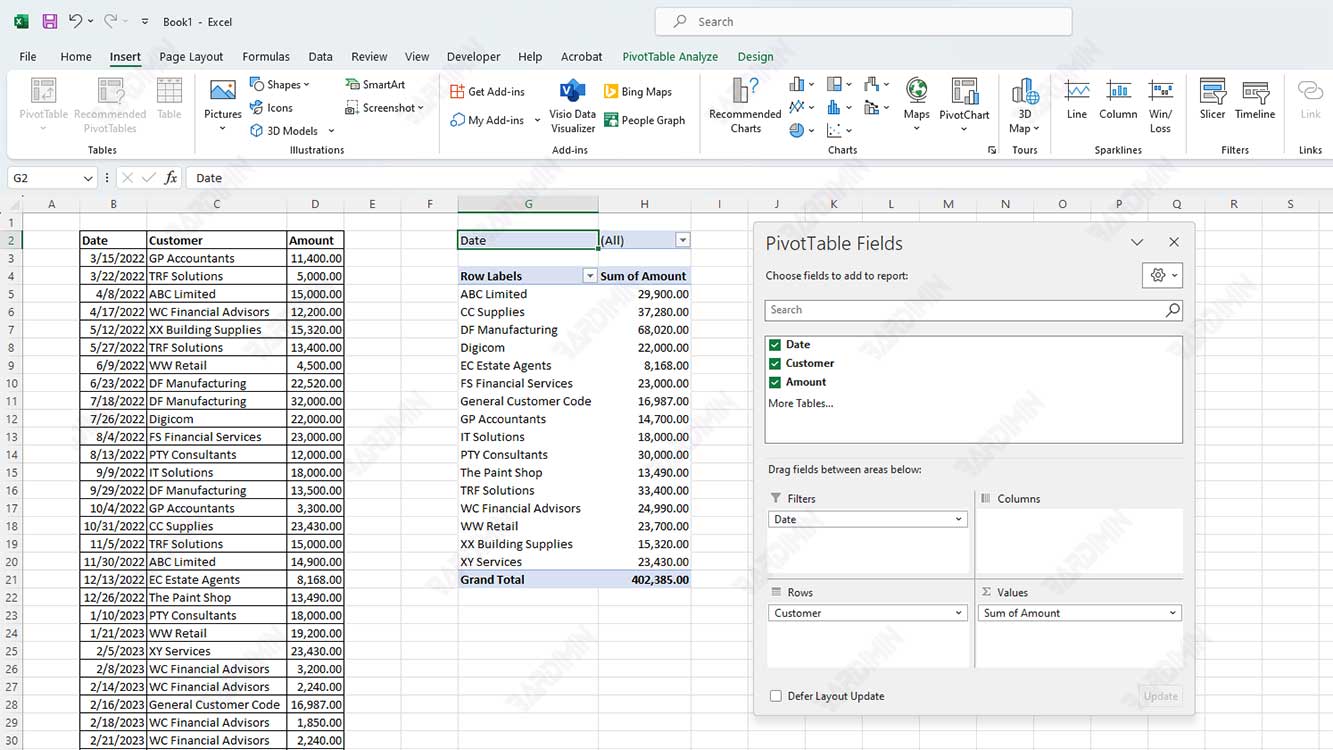
3] Pivot Table Report
You can see an example of a Pivot Table in the below screenshot. You can select an option from the list by clicking the dropdown button. Choose what you want to display on the page by selecting it from the list. You can select “All” to see everything.