How to Draw a Perfect Circle in Excel

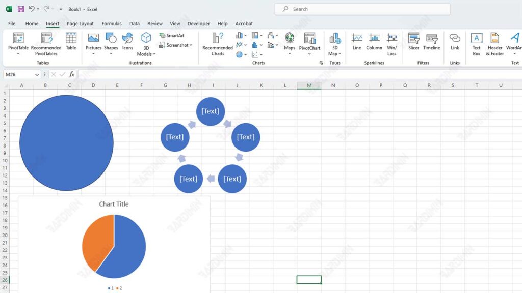
Have you ever wanted to create a perfect circle in Excel? Maybe you want to create pie charts, pie charts, or just simply decorate your worksheet with geometric shapes. Whatever your reason, you may find that it is difficult to draw a complete circle in Excel. If you use the built-in Shape tool, you may get an unsymmetrical ellipse or oval. If you try to set the size and position of the Shape manually, you may spend a lot of time and still not get the desired results.

So, how to draw a perfect circle in Excel? Is there any trick or formula you can use? The answer is yes, there are several ways you can try to create a perfect and neat circle in Excel. In this article, Bardimin will show you three different methods to draw circles in Excel, namely:

• Using the Shape tool by pressing the Shift button
• Use SmartArt tools by selecting Cycle
• Use the Chart tool by creating a Pie Chart

Let’s look at each of the methods in more detail.

Use the Shape tool by pressing the Shift key

One of the easiest ways to draw a perfect circle in Excel is to use the Shape tools available in the Insert tab. However, you should be careful when selecting and dragging Shape in your worksheet. If you just draw Shape randomly, you may get a shape that is not round. To avoid this, press and hold the Shift button while dragging the Shape. This will ensure that your Shape has a 1:1 aspect ratio, which means the width and height are the same.

Here are the steps to draw a perfect circle using the Shape tool and the Shift button:

1. Open the Excel worksheet to which you want to add circles.
2. Click the Insert tab in the ribbon, and then click the Shapes icon in the Illustrations group.
3. From the drop-down menu that appears, select Oval under the Basic Shapes category.
4. Hover your cursor over any cell in your worksheet, and then press and hold the Shift key on your keyboard.
5. While holding down the Shift key, click and drag your cursor to create a circle. You’ll see a dotted line that shows the shape of your circle.
6. Release the Shift button and click your mouse when you are satisfied with the size and position of your circle.
7. You can change the color, outline, effects, and other properties of your circle by using the Format tab under Shape Tools.

Use SmartArt tools by selecting Cycle

Another way to draw a perfect circle in Excel is to use the SmartArt tool, which is also available in the Insert tab. The SmartArt tool allows you to create different graphs and diagrams that are attractive and informative. One type of SmartArt that you can use to create circles is Cycle. Cycle is a category of SmartArt that displays an iterative or continuous process using circle shapes.

Here are the steps to draw a perfect circle by using the SmartArt tool and selecting Cycle:

1. Open the Excel worksheet to which you want to add circles.
2. Click the Insert tab in the ribbon, and then click the SmartArt icon in the Illustrations group.
3. From the Choose a SmartArt Graphic dialog box that appears, select Cycle under the Process category.
4. You’ll see several different Cycle design options. Choose the one that suits your needs. For example, if you want to create a single circle, you can select Basic Cycle. If you want to create multiple interconnected circles, you can choose Continuous Cycles or Interlocking Cycles.
5. Click OK to insert SmartArt into your worksheet.
6. You can adjust the size, position, color, style, and text of your circles by using the Design and Format tabs under SmartArt Tools.

Using the Chart tool by creating a Pie Chart

The third way to draw a perfect circle in Excel is to use the Chart tool which is also available in the Insert tab. The Chart tool allows you to create different types of graphs and graphs that can display your data visually. One type of Chart you can use to create circles is the Pie Chart. A Pie Chart is a type of graph that displays the proportion of your data in the form of circular slices.

Here are the steps to draw a perfect circle using the Chart tool and create a Pie Chart:

1. Open the Excel worksheet to which you want to add circles.
2. Create a simple data table that contains two columns. The first column contains your data labels, and the second column contains the values of your data. Make sure the sum of your data values equals 100, as this will represent the total percentage of your circles.
3. Select your entire data table, then click the Insert tab in the ribbon.
4. Click the Pie icon in the Charts group, then select one of the available Pie Chart types. For example, you can select a 2-D Pie or 3-D Pie.
5. Excel will create a Pie Chart based on your data and insert it into your worksheet.
6. You can adjust the size, position, color, legend, labels, and other properties of your circles by using the Design and Format tabs under Chart Tools.

Conclusion

In this article, you have learned three different ways to draw a perfect circle in Excel, namely:

• Using the Shape tool by pressing the Shift button
• Use SmartArt tools by selecting Cycle
• Use the Chart tool by creating a Pie Chart

All of these methods have their advantages and disadvantages, depending on your goals and preferences. You can try and compare these methods to find the one that works best for you. With a little practice and creativity, you can create perfect and interesting circles in Excel.