PivotTables are a great feature in Microsoft Excel that is built to summarize, analyze, and present data in an easier way. With PivotTable, users can rearrange data without changing the source, making it easier to explore from multiple perspectives.
The four main areas in the PivotTable, namely the Values Area, the Row Area, the Column Area, and the Filter Area, are critical components that enable flexible and in-depth data analysis. Understanding the functions of each area helps the user:
- Segment data effectively.
- Analyze the numbers most appropriately.
- Customize the view of data according to business needs or reports.
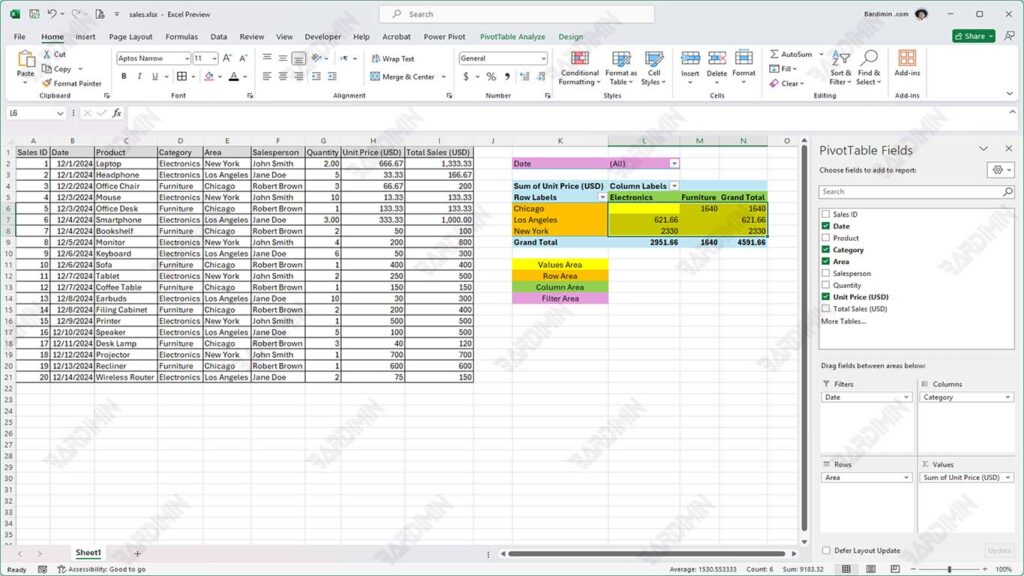
Four Key Areas in the PivotTable
1. Values Area
The Values Area is a key component in a PivotTable that is used to calculate and display numerical data, such as Revenue, Count of Units, or Average of Price. This area presents the results of the analysis in the form of numbers that are easy to understand and allow users to conduct quantitative analysis of existing data.
For example, if you have product sales data, you can use the Values Area to display the total sales of each product category. This way, you can quickly see which categories are contributing the most to revenue.
Tips:
- Use aggregation: Choose an aggregation method that suits your analysis needs, such as Sum for the total, Count for the number of entries, or Average for the average.
- Add number formatting: Setting the number format (for example, currency or percentage) can make the data easier for users to read and understand.
2. Row Area
Row Areas in a PivotTable are used to group data based on a specific category, such as Product, Name, or Location. With Row Areas, users can view data in a more structured way, making it easy to analyze and compare between categories.
For example, you can create a sales table by product category. By placing product categories in the Row Area, you can easily see the total sales for each category, which helps in understanding the performance of each product.
Tips
- Use organized data: Sorting your data before creating a PivotTable will give you a cleaner and more organized look. It also makes it easier to find certain information.
- Make sure each column has a clear title: A clear and descriptive title is essential for understanding the context of the data. It is also helpful when sharing reports with others so that they can quickly understand the contents of the table.
3. Column Area
The Column Area in a PivotTable is used to display data in the form of columns. It is often used to show time trends or create matrix data. With the Column Area, users can compare and analyze data from a column perspective, making it easier to see patterns and changes over time.
For example, you can view sales data per month. By placing the month in the Column Area, you can see how sales change each month, providing information about seasonal trends or monthly performance.
Tips
- Great for comparing trends between categories: Column Areas are especially useful when you want to see comparisons between categories in the context of time or other parameters. For example, comparing sales of products A and B from month to month.
- Combine with charts for data visualization: Using charts with PivotTables can improve visual understanding of data. Charts such as bar or line charts can provide a clearer picture of trends and comparisons.
4. Filter Area
The Area Filter in the PivotTable allows users to filter the data to make the analysis more focused. With Area Filters, users can select specific criteria that they want to display, allowing them to gain deeper insights from relevant data.
For example, you can show sales only for a specific region. By applying filters to those regions, you can analyze sales performance in that area without being distracted by data from other regions.
Tips
- Add Slicers for easier navigation: Slicers are visual tools that make it easy for users to select and apply filters. With the addition of Slicer, interacting with data becomes more intuitive and faster.
- Use filters on important categories, such as time or location: Focusing filters on significant categories, such as time range or location, will help in getting more relevant and useful insights.
How to Use the 4 Areas in a PivotTable
1. Select Data and Create a PivotTable
The first step is to select the data you want to analyze. Make sure the data is well-organized and has clear headers for each column. After selecting the data, go to the Insert tab in Microsoft Excel and select PivotTable. In the window that appears, select a location for the new PivotTable, either in the same worksheet or in the new worksheet.
2. Drag and Drop Data to Each Area
Once the PivotTable is created, you will see the PivotTable Fields panel. Here, you can drag and drop data to each area:
- Enter numeric data into the Values Area: Drag columns that contain numerical data (such as sales or revenue) to the Values Area. It allows you to calculate the total, average, or number of units.
- Add a primary category to the Row Area: Drag the column containing the primary category (such as the product name or location) to the Row Area. This will group the data based on those categories.
- Use Column Area for data comparison: If you want to compare data based on a specific parameter (for example, time), drag the column to the Column Area. It helps you see the comparison between categories in a column format.
- Use Area Filter to focus on a subset of data: Drag the column you want to use as a filter (such as a region or period) to Filter Area. This allows you to filter the data and focus on a specific subset.
3. Adjust Format and Aggregation as Needed
Once all the data is in the right place, the final step is to adjust the format and aggregation according to your analysis needs:
- Set number format: Right-click on a value in the Value Area and select Value Field Settings to change the aggregation method (Sum, Calculate, Average) according to the analysis needs.
- Apply visual formatting: Use formatting options in Excel to change the appearance of numbers to make them easier to read, such as adding currency symbols or setting decimal numbers.